Warning in fun(libname, pkgname): mzR has been built against a different Rcpp version (1.0.14)
than is installed on your system (1.1.0). This might lead to errors
when loading mzR. If you encounter such issues, please send a report,
including the output of sessionInfo() to the Bioc support forum at
https://support.bioconductor.org/. For details see also
https://github.com/sneumann/mzR/wiki/mzR-Rcpp-compiler-linker-issue.
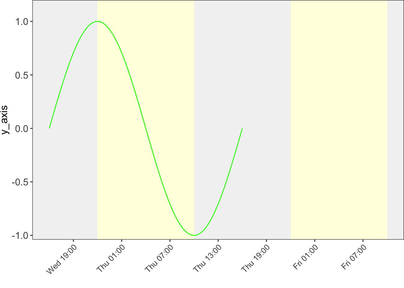
By using the time_plot function, you can obtain the visualization results of the time series.
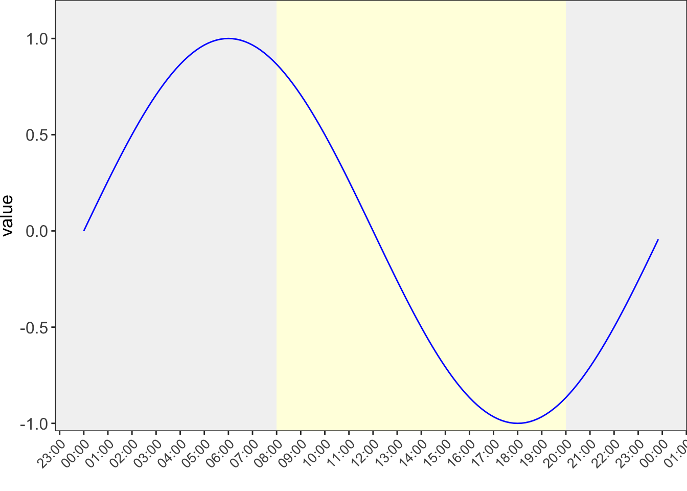
This chunk creates a small, clean time series suitable for lagged-correlation demos.
It builds a datetime column as a POSIXct sequence from 2003-01-09 00:00:00 to 2003-01-10 00:00:00 at 10-minute intervals, then computes a smooth sine wave over the full range 0→2π0 →2π with exactly nrow(example_data_1) points, storing it in value.
Because seq(..., by = "10 min") controls the sampling, you get evenly spaced timestamps; the data are deterministic (no randomness), so results are reproducible. head(example_data_1) just previews the first few rows.
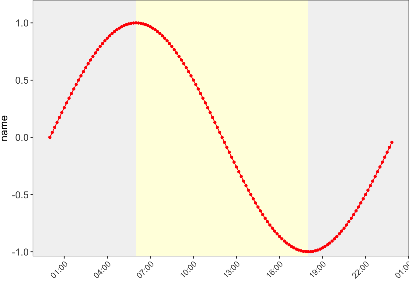
For downstream analysis, most lag tools expect columns named time (POSIXct) and value. You can simply rename with dplyr::rename(example_data_1, time = datetime), and—if you need cross-machine consistency—set an explicit timezone when creating the sequence (e.g., as.POSIXct(..., tz = "UTC")).
example_data_1<-data.frame( datetime =seq(from =as.POSIXct("2003-01-09 00:00:00"), to =as.POSIXct("2003-01-10 00:00:00"), by ="10 min"))example_data_1$value<-sin(seq(from =0, to =2*pi, length.out =nrow(example_data_1)))head(example_data_1)